Contents

Build a PLS regression model

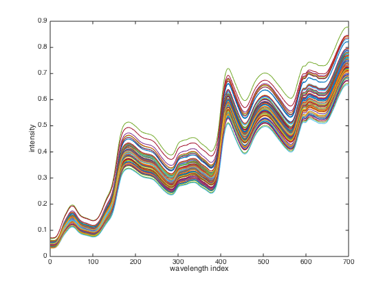
This example illustrates how to build a PLS model using a benchmark NIR data.

%cd /Users/hdl/Documents/Study/MATLAB/libPLS/libPLS_dev  % first go to the
%  folder of libPLS.
%**************************************************
%**********   NOTES  ******************************
%** MAKE SURE to go to your OWN libPLS folder  ****
%**************************************************

clear;
load corn_m51;          % example data

close(gcf);
plot(X');               % display spectral data.
xlabel('wavelength index');
ylabel('intensity');

parameter setting

A=6;                    % number of latent variables (LVs).
method='center';        % internal pretreatment method of X for building PLS model
PLS=pls(X,y,A,method);  % command to build a model

PLS

PLS = 

                  method: 'center'
              X_pretreat: [80x700 double]
              y_pretreat: [80x1 double]
        regcoef_pretreat: [700x1 double]
    regcoef_original_all: [701x6 double]
        regcoef_original: [701x1 double]
                X_scores: [80x6 double]
              X_loadings: [700x6 double]
                     VIP: [1x700 double]
                       W: [700x6 double]
                   Wstar: [700x6 double]
                   y_fit: [80x1 double]
                fitError: [80x1 double]
                tpscores: [80x1 double]
              tploadings: [700x1 double]
                      SR: [1x700 double]
                     SST: 11.4295
                     SSR: 11.3476
                     SSE: 0.0820
                   RMSEF: 0.0320
                      R2: 0.9928

The pls.m function returns an object PLS containing a list of components: Results interpretation:

     regcoef_original: regression coefficients that links X and y.
     X_scores: scores of X
     VIP: variable importance in projection, a criterion for assessing
     importance of variables
     RMSEF: root mean squared errors of fitting.
     y_fit: fitted values of y.
     R2: percentage of explained variances of y.

K-fold cross validation of PLS

Illustrate how to perform K-fold cross validation of PLS models

clear;
load corn_m51;                % example data
A=6;                          % number of LVs
K=5;                          % fold number for cross validations
method='center';
CV=plscv(X,y,A,K,method);

The 1th group finished.
The 2th group finished.
The 3th group finished.
The 4th group finished.
The 5th group finished.

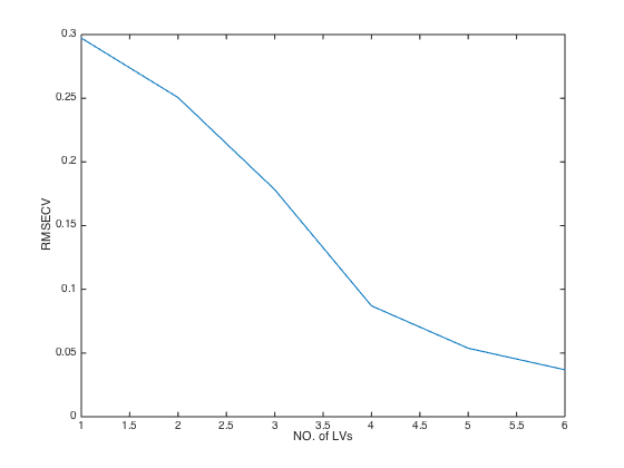
close(gcf)
plot(CV.RMSECV)               % plot RMSECV values at each number of latent variables(LVs)
xlabel('NO. of LVs')          % add X label
ylabel('RMSECV')              % add Y label

CV

CV = 

            method: 'center'
             Ypred: [80x6 double]
         predError: [80x6 double]
            RMSECV: [0.2972 0.2505 0.1782 0.0870 0.0538 0.0369]
                Q2: [0.3816 0.5606 0.7777 0.9470 0.9798 0.9905]
        RMSECV_min: 0.0369
            Q2_max: 0.9905
             optLV: 6
              note: '*** The following is based on global min MSE + 1SD'
    RMSECV_min_1SD: 0.0538
        Q2_max_1SD: 0.9798
         optLV_1SD: 5

The returned value CV is structural data with a list of components: Results interpretation:

     RMSECV: root mean squared errors of cross validation. The smaller,
     the better
     Q2: same meaning as R2 but calculated from cross validation.
     optLV: the number of LVs that achieves the minimal RMSECV (the highest Q2)

Monte Carlo cross validation (MCCV) of PLS

Illustrate how to perform MCCV for PLS modeling. like K-fold CV, MCCV is another approach for cross validation.

clear;
load corn_m51;                  % example data

% parameter settings
A=6;
method='center';
N=500;                          % number of Mnote Carlo sampings.
MCCV=plsmccv(X,y,A,method,N);   % run MCCV

The 100th sampling for MCCV finished.
The 200th sampling for MCCV finished.
The 300th sampling for MCCV finished.
The 400th sampling for MCCV finished.
The 500th sampling for MCCV finished.

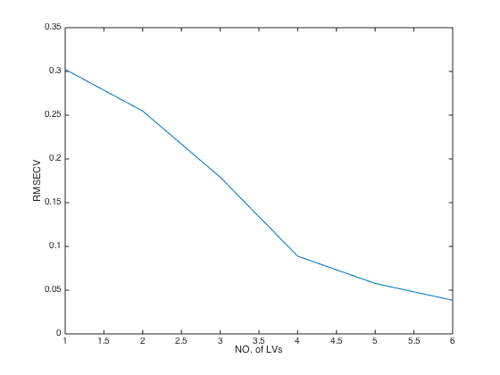
close(gcf);
plot(MCCV.RMSECV);              % plot RMSECV values at each number of latent variables(LVs)
xlabel('NO. of LVs');
ylabel('RMSECV');

MCCV

MCCV = 

            method: 'center'
           MC_para: [500 0.8000]
             Ypred: [8000x6 double]
             Ytrue: [8000x1 double]
            RMSECV: [0.3023 0.2547 0.1792 0.0889 0.0577 0.0385]
        RMSECV_min: 0.0385
                Q2: [0.3625 0.5475 0.7761 0.9449 0.9768 0.9897]
            Q2_max: 0.9897
             optLV: 6
             RMSEF: [500x6 double]
             RMSEP: [500x6 double]
              note: '****** The following is based on global min MSE + 1SD'
    RMSECV_min_1SD: 0.0577
        Q2_max_1SD: 0.9768
         optLV_1SD: 5
              time: 1.4960

MCCV is an structural data. Results interpretation:

     Ypred:predicted values
     Ytrue: real values
     RMSECV: root mean squared errors of cross validation. The smaller,
     the better
     Q2: same meaning as R2 but calculated from cross validation.

Double cross validation (DCV) of PLS

Illustrate how to perform DCV for PLS modeling. like K-fold CV, DCV is a way for cross validation.

clear;
load corn_m51;                        % example data

% parameter settings
A=6;
k=5;
method='center';
N=50;                                 % number of Mnote Carlo sampings
DCV=plsdcv(X,y,A,k,method,N);

DCV

DCV = 

       method: 'center'
       RMSECV: 0.0369
          nLV: [5x1 double]
        RMSEP: [5x1 double]
    predError: [80x1 double]

Outlier detection using the Monte Carlo sampling approach

Illustrate the use of an outlier detection method

clear;
load corn_m51; % example data
A=6;
method='center';
N=1000;
ratio = 0.7;
F=mcs(X,y,A,method,N,ratio);

The 100/1000th MCS finished.
The 200/1000th MCS finished.
The 300/1000th MCS finished.
The 400/1000th MCS finished.
The 500/1000th MCS finished.
The 600/1000th MCS finished.
The 700/1000th MCS finished.
The 800/1000th MCS finished.
The 900/1000th MCS finished.
The 1000/1000th MCS finished.

F

F = 

         pretreat: 'center'
    MCS_parameter: [1000 0.7000]
        predError: [1000x80 double]
             MEAN: [1x80 double]
              STD: [1x80 double]

Results interpretation:

     predError: prediction errors of the samples in each sampling
     MEAN: mean predidction errors of each sample
     STD:standard deviation of prediction errors of each sample

close(gcf)
plotmcs(F) % Diagnostic plots

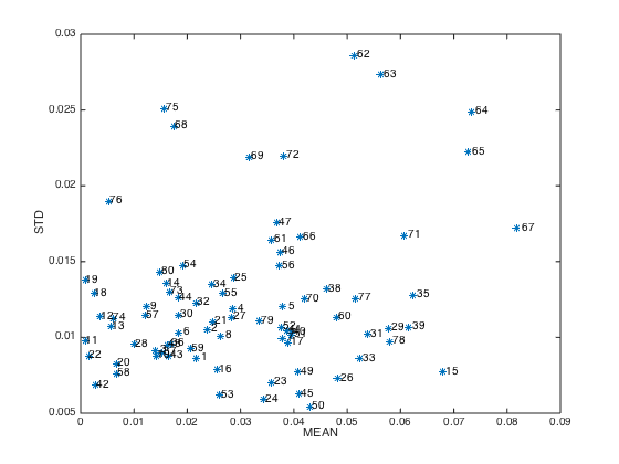
Notes: samples with high MEAN or high SD are more likely to be outliers and should be considered to be removed before modeling.

Variable selection using the CARS method.

clear;
load corn_m51;                      % example data
A=6;
fold=5;
CARS=carspls(X,y,A,fold);

Sampling...
Evaluating...
Done...

CARS

CARS = 

             W: [700x50 double]
          time: 0.4639
        RMSECV: [1x50 double]
    RMSECV_min: 2.9460e-04
        Q2_max: 1.0000
       iterOPT: 49
         optLV: 2
         ratio: [1x50 double]
          vsel: [405 505]

Results interpretation:

     optLV:number of LVs of the best model
     vsel: selected variables (columns in X)

close(gcf)
plotcars(CARS); % Diagnostic plots

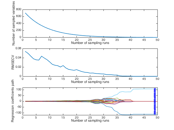
Note: in this plot,the top and middle panel shows how the number of selecte variables and RMSECV change with interations. The bottom panel describes how regression coefficients of each variable(each line corresponds to a variable) change with iterations. The star vertical line indiciates the best model with the lowest RMSECV.

Variable selection using moving window PLS (MWPLS).

clear;
load corn_m51;                      % example data
A=6;
width=15;                           % window size
[WP,RMSEF]=mwpls(X,y,A,width);

close(gcf);
plot(WP,RMSEF);
xlabel('Window position');
ylabel('RMSEF')

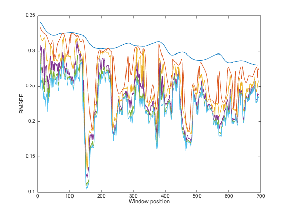
Note: From this plot, regions with low RMSEF values are recommended to be included in a PLS model

Variable selection using Monte Carlo Uninformative Variable Elimination (MCUVE)

clear;
load corn_m51;                      % example data
A=6;
N=500;
method='center';
UVE=mcuvepls(X,y,A,method,N);

The 100/500th sampling for MC-UVE finished.
The 200/500th sampling for MC-UVE finished.
The 300/500th sampling for MC-UVE finished.
The 400/500th sampling for MC-UVE finished.
The 500/500th sampling for MC-UVE finished.

UVE

UVE = 

                RI: [1x700 double]
    SortedVariable: [1x700 double]
           regcoef: [500x700 double]
              MEAN: [1x700 double]
                SD: [1x700 double]

close(gcf);
plot(abs(UVE.RI))

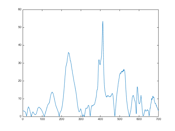
Results interpretation: RI: reliability index of UVE, a measurement of variable importance. The higher, the better.

Variable selection using Random Frog

clear;
load corn_m51;                      % example data
A=6;
N=10000;
method='center';
FROG=randomfrog_pls(X,y,A,method,N);

The 1000th sampling for random frog finished.
The 2000th sampling for random frog finished.
The 3000th sampling for random frog finished.
The 4000th sampling for random frog finished.
The 5000th sampling for random frog finished.
The 6000th sampling for random frog finished.
The 7000th sampling for random frog finished.
The 8000th sampling for random frog finished.
The 9000th sampling for random frog finished.
The 10000th sampling for random frog finished.
Elapsed time is 40.095188 seconds.

FROG

FROG = 

              N: 10000
              Q: 2
          model: [10000x700 double]
        minutes: 0.6683
         method: 'center'
          Vrank: [1x700 double]
         Vtop10: [505 405 506 400 408 233 235 249 248 515]
    probability: [1x700 double]
           nVar: [1x10000 double]
          RMSEP: [1x10000 double]

close(gcf);
plot(FROG.probability)
xlabel('variable index');
ylabel('selection probability');

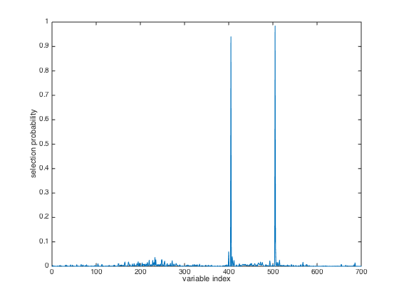
Results interpretation:

    model: a matrix storing the selecte variables at each interation
    probability: the probability of each variable to be included in a
    final model. The larger, the better. This is a useful metric to
    measure variable importance.

Published with MATLAB® R2014b