Contents
- Build a PLS-LDA model
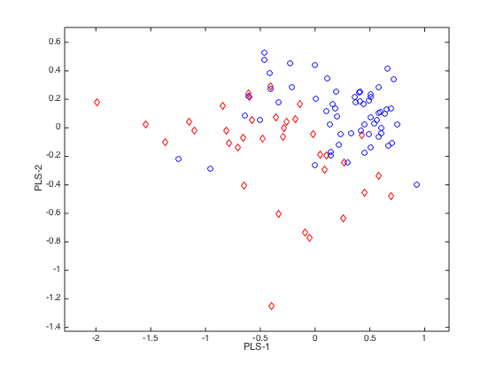
- Visualization of a PLS-LDA model with two latent variables
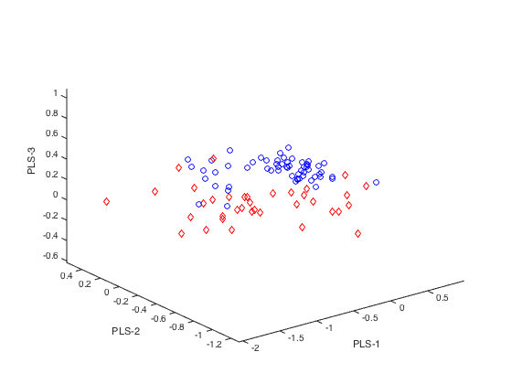
- Visualization of a PLS-LDA model with three latent variables
- K-fold cross validation of PLSLDA
- Monte Carlo cross validation (MCCV) of PLS-LDA
- Variable selection using the original CARS method described in our CARS paper.
- Variable selection using a simplified version of CARS where the built-in
- Variable selection using Random Frog
- Variable selection using Subwindow Permutation Analysis (SPA)
- Variable selection using PHADIA (Phase Diagram)
Build a PLS-LDA model
This example illustrates how to build a PLS-LDA model using a demo metabolomic data.
%cd /Users/hdl/Documents/Study/MATLAB/libPLS/libPLS_dev  % first go to the
%  folder of libPLS.
clear;
load DM2;                     % example data
A=3;                          % number of latent variables (LVs).
method='center';              % internal pretreatment method of X for building PLS-LDA model
PLSLDA=plslda(X,y,A,method);  % command to build a model
PLSLDA
PLSLDA =

                method: 'center'
            scale_para: [2x40 double]
                 yreal: [96x1 double]
      regcoef_pretreat: [40x1 double]
                   VIP: [1x40 double]
                 Wstar: [40x3 double]
                     W: [40x3 double]
               Xscores: [96x3 double]
             Xloadings: [40x3 double]
                   R2X: [3x1 double]
                   R2Y: [3x1 double]
              tpScores: [96x1 double]
            tpLoadings: [40x1 double]
                    SR: [1x40 double]
                   LDA: '*********  LDA ***********'
        regcoef_lda_lv: [4x1 double]
    regcoef_lda_origin: [41x1 double]
                  yfit: [96x1 double]
                 error: 0.0833
           sensitivity: 0.9500
           specificity: 0.8611
                   AUC: 0.9435
PLSLDA is a structural data Results interpretation:
     Xscores:scores of X matrix
     regcoef_lda_origin:regression coefficients of variables in X. The
     last column is the intercept.
     error: fitting errors on training data.
Visualization of a PLS-LDA model with two latent variables
This example illustrates how to build a PLS-LDA model using a demo metabolomic data.
%cd /Users/hdl/Documents/Study/MATLAB/libPLS/libPLS_dev  % first go to the
%  folder of libPLS.

clear;
load DM2;                       % example data
A=2;                            % number of latent variables (LVs).
method='center';                % internal pretreatment method of X for building PLS-LDA model
PLSLDA=plslda(X,y,A,method);    % command to build a model
close(gcf)
plotlda(PLSLDA,0,0,[1,2]) % plot samples in PLS component space
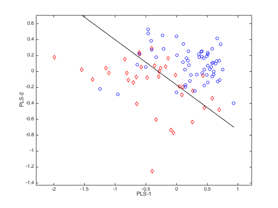
close(gcf)
plotlda(PLSLDA,0,1,[1,2]) % plot samples in PLS component space with separating line shown.
Visualization of a PLS-LDA model with three latent variables
This example illustrates how to build a PLS-LDA model using a demo metabolomic data.
%cd /Users/hdl/Documents/Study/MATLAB/libPLS/libPLS_dev  % first go to the
%  folder of libPLS.
clear;
load DM2;                       % example data
A=3;                            % number of latent variables (LVs).
method='center';                % internal pretreatment method of X for building PLS-LDA model
PLSLDA=plslda(X,y,A,method);    % command to build a model
close(gcf)
plotlda(PLSLDA,0,0,[1,2,3])     % with no separating plain
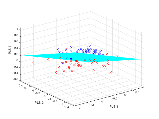
close(gcf)
plotlda(PLSLDA,0,1,[1,2,3])     % with separating plane
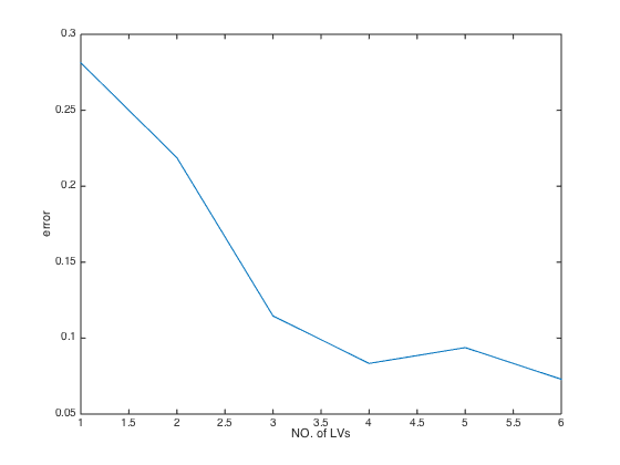
K-fold cross validation of PLSLDA
Illustrate how to perform K-fold cross validation of PLS-LDA models
load DM2;                       % example data
A=6;                            % number of LVs
K=5;                            % fold number for cross validations
method='center';
CV=plsldacv(X,y,A,K,method);
The 1th fold for PLS-LDA finished.
The 2th fold for PLS-LDA finished.
The 3th fold for PLS-LDA finished.
The 4th fold for PLS-LDA finished.
The 5th fold for PLS-LDA finished.
CV
CV =

         method: 'center'
          Ypred: [96x6 double]
              y: [96x1 double]
          error: [0.2812 0.2188 0.1146 0.0833 0.0938 0.0729]
      error_min: 0.0729
          optLV: 6
    sensitivity: 0.9500
    specificity: 0.8889
            AUC: 0.9889
Results interpretation:
     RMSECV: root mean squared errors of cross validation. The smaller,
     the better
     Q2: same meaning as R2 but calculated from cross validation.
     optLV: the number of LVs that achieves the minimal RMSECV (the highest Q2)
close(gcf) plot(CV.error); % plot RMSECV values at each number of latent variables(LVs) xlabel('NO. of LVs') % add X label ylabel('error') % add Y label
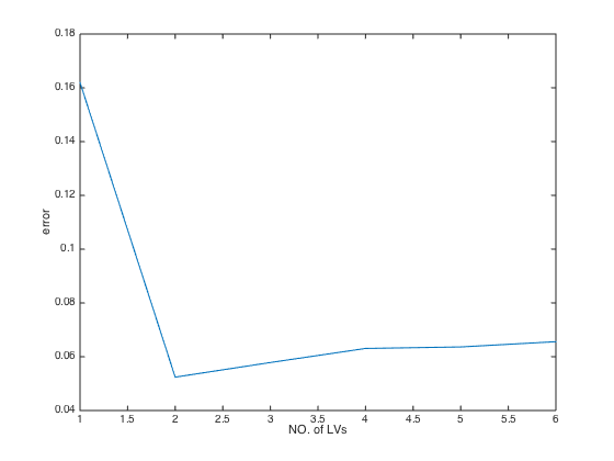
Monte Carlo cross validation (MCCV) of PLS-LDA
Illustrate how to perform MCCV for PLS-LDA modeling. like K-fold CV, MCCV is another approach for cross validation.
clear;
load DM2;                           % example data
% parameter settings
A=6;
method='center';
N=500;                              % number of Mnote Carlo sampings.
ratio=0.6;
MCCV=plsldamccv(X,y,A,N,ratio);
MCCV
MCCV =

       method: 'autoscaling'
        error: [0.1619 0.0524 0.0578 0.0631 0.0636 0.0656]
    error_min: 0.0524
        optLV: 2
Results interpretation:
     error: cross-validated errors at each number of LV
     error_min: the min errors
     optLV: the optimal number of LVs selected by MCCV
close(gcf); plot(MCCV.error); % plot RMSECV values at each number of latent variables(LVs) xlabel('NO. of LVs'); ylabel('error');
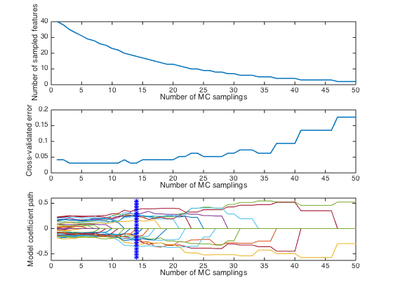
Variable selection using the original CARS method described in our CARS paper.
clear
load DM2;                           % example data
A=6;
fold=5;
N=50;
CARS=carsplslda(X,y,A,fold,N);
CARS
CARS =

       method: 'autoscaling'
            W: [50x40 double]
        error: [1x50 double]
    error_min: 0.0312
      iterOPT: 14
        optLV: 6
        ratio: [1x50 double]
         vsel: [18x1 double]
Results interpretation:
     optLV:number of LVs of the best model
     vsel: selected variables (columns in X)
Diagnostic plots
close(gcf)
plotcars_plslda(CARS);

% Notes: in this plot,the top and middle panel shows how the number of selecte
% variables and RMSECV change with interations. The bottom panel describes
% how regression coefficients of each variable(each line corresponds to
% a variable) change with iterations. The star vertical line indiciates the
% best model with the lowest RMSECV.
Variable selection using a simplified version of CARS where the built-in
randomized sampling component was removed. So, each run of CARS will
give the same results.
clear
load DM2;                           % example data
A=6;
fold=5;
N=50;
CARS=carsplslda(X,y,A,fold,N,'center',0);
CARS
CARS =

       method: 'center'
            W: [50x40 double]
        error: [1x50 double]
    error_min: 0.0312
      iterOPT: 15
        optLV: 4
        ratio: [1x50 double]
         vsel: [17x1 double]
Results interpretation:
     optLV:number of LVs of the best model
     vsel: selected variables (columns in X)
% Diagnostic plots
close(gcf)
plotcars_plslda(CARS);
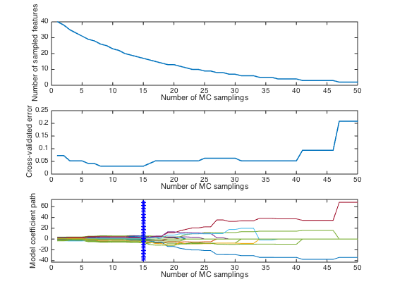
Notes: in this plot,the top and middle panel shows how the number of selecte variables and RMSECV change with interations. The bottom panel describes how regression coefficients of each variable(each line corresponds to a variable) change with iterations. The star vertical line indiciates the best model with the lowest RMSECV.
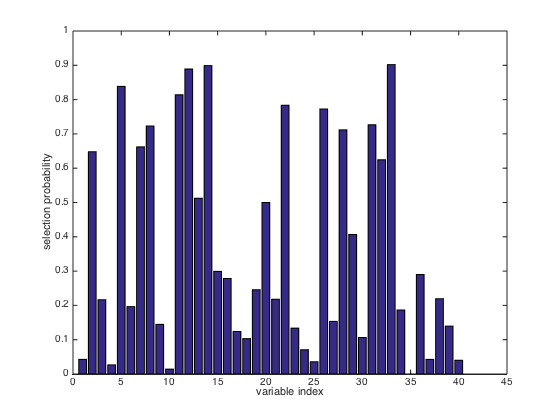
Variable selection using Random Frog
clear;
load DM2;                              % example data
A=6;
N=2000;
method='center';
FROG=randomfrog_plslda(X,y,A,method,N);
The 1000th sampling for random frog finished.
The 2000th sampling for random frog finished.
Elapsed time is 25.414775 seconds.
FROG
FROG =

              N: 2000
              Q: 2
        minutes: 0.4236
         method: 'center'
          Vrank: [1x40 double]
         Vtop10: [33 14 12 5 11 22 26 31 8 28]
    probability: [1x40 double]
           nVar: [1x2000 double]
          RMSEP: [1x2000 double]
Results interpretation:
    Vrank: the top ranked variables. The first one is the most
    important.
    probability: the probability of each variable to be included in a
    final model. The larger, the better. This is a useful metric to
    measure variable importance.
close(gcf) bar(FROG.probability) xlabel('variable index'); ylabel('selection probability');
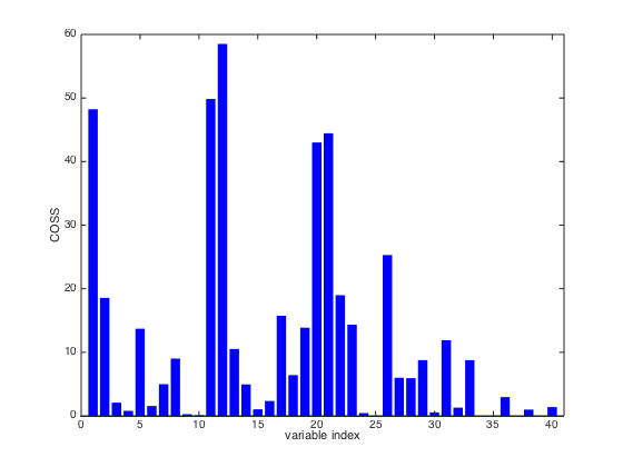
Variable selection using Subwindow Permutation Analysis (SPA)
clear;
load DM2;                           % example data
A=6;
K=3;                                % fold for cross validation
Q=10;                               % window size, e.g. the number of variables included in a sub-model
ratio=0.6;                          % ratio of samples to be used as training data for each sub-model
N=1000;
method='center';
SPA=spa(X,y,A,K,Q,N,ratio,method);
Elapsed time is 6.014934 seconds.
SPA
SPA =

            method: 'center'
              time: 0.1002
                 N: 1000
             ratio: 0.6000
                 Q: 10
               nLV: [1000x1 double]
               NPE: [1000x1 double]
               PPE: [1000x40 double]
             DMEAN: [40x1 double]
               DSD: [40x1 double]
          interfer: [1x40 double]
                 p: [1x40 double]
              COSS: [1x40 double]
    RankedVariable: [1x40 double]
Results interpretation:
    p:p-value mesuring the significance of variables. Note that for
    variables inclusion of which would reduce model performances,the
    p-value is added by one. So, it is a pseudo-pvalue here.
    COSS: COnditional Synergistic Score, this is the key output of SPA
    and used to rank variables.
% COSS is calculated as COSS=-log10(pvalue). So a pvalue=0.05, is % corresponding to COSS value= 1.3. COSS for pvalue=0.01 is 2.
close(gcf)
bar(SPA.COSS,'edgecolor','none','facecolor','b')
xlim([0 41])
xlabel('variable index');
ylabel('COSS');
Variable selection using PHADIA (Phase Diagram)
clear;
load DM2;                           % example data
A=6;
K=3;                                % fold for cross validation
Q=10;                               % window size, e.g. the number of variables included in a sub-model
ratio=0.6;                          % ratio of samples to be used as training data for each sub-model
N=1000;
method='center';
PHADIA=phadia(X,y,A,method,N,Q,K);
The 100/1000th sampling for variable selection finished.
The 200/1000th sampling for variable selection finished.
The 300/1000th sampling for variable selection finished.
The 400/1000th sampling for variable selection finished.
The 500/1000th sampling for variable selection finished.
The 600/1000th sampling for variable selection finished.
The 700/1000th sampling for variable selection finished.
The 800/1000th sampling for variable selection finished.
The 900/1000th sampling for variable selection finished.
The 1000/1000th sampling for variable selection finished.
***>>> Evaluating variable importance...
***>>> Evaluating finished.
***>>> PS: Variable Selection based on Model Population Analysis.
Elapsed time is 4.455757 seconds.
PHADIA
PHADIA =

               method: 'center'
    parameter_meaning: 'N Q K'
           parameters: [1000 10 3]
          TimeMinutes: 0.0743
                model: {1x40 cell}
                  nLV: [1000x1 double]
            PredError: [1000x1 double]
                DMEAN: [1x40 double]
                  DSD: [1x40 double]
                    p: [1x40 double]
Results interpretation:
p:p-value mesuring the significance of variables.
close(gcf);
plotphadia(PHADIA);                 % a 2D diagram for visualizing predictive ability of all variables.
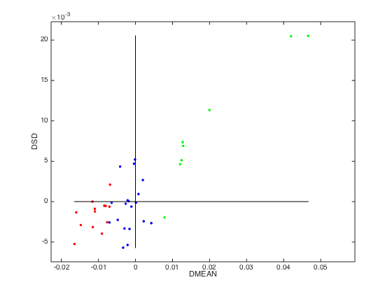
     Notes:
     On the 2D plot below, the green dots indicate good variables inclusion of
     which would on average increase model performance; red dots
     indicate 'bad' variables, inclusion of which would on average
     decrease model performance; blue dots indicate noisy variables,
     inclusion of which have no significant effects to model
     performance.